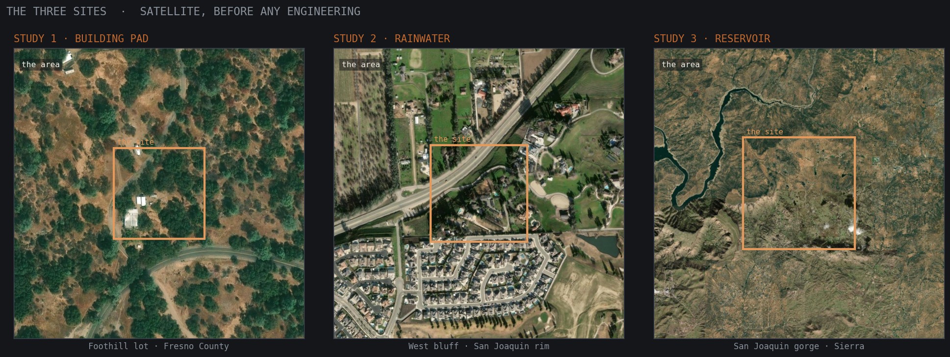
← Back to the portfolio
Project
Terrain studies
Subject
Three
Sierra sites
Source
USGS 3DEP
10 m NED
Surface
Delaunay TIN
Engine
planar-
geometry
Prepared
H. Wolf
2026-07-07
Terrain & earthwork · three studies

What can the engines really do?

Three preliminary terrain questions: how much earth a level pad would move on a sloped foothill lot; where a storm would run across a bluff; and how much water a dammed Sierra canyon would hold. The studies were computed in about an hour and a half using two existing systems that were not built for terrain (how this was built, below).

Computed end to end from public 10 m USGS elevation; proofs of concept rather than a survey. Method · The engines behind it
01Study 1 · Building padFoothill lot · Fresno County · 37.08°N 119.49°W

Imagine a lot for sale in the foothills. You want to buy it and build a house, but the ground sits on a slope. How steep, exactly? How hard would it be to get a pad level, and how much dirt would have to be cut, filled, or trucked out to do it? You can't eyeball any of that, and it's most of the grading bill. It's the number you'd want before you make the offer: what does a level pad here cost in dirt?
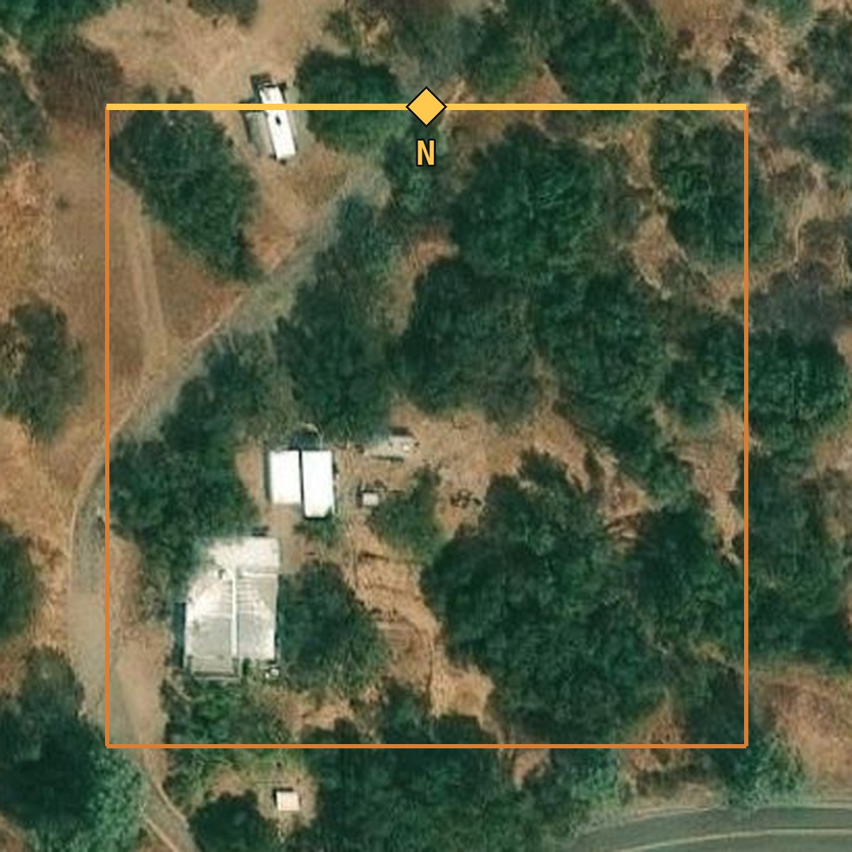
Plain satellite view of the foothill lot, the kind of map view a buyer would pull up online.
the lot, from the map
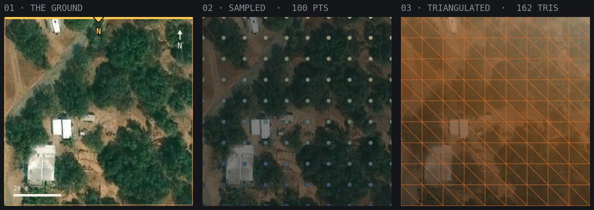
Build maps of the site: the satellite with the study boundary, its marked edge badged with its cardinal letter, the sampled points, and the mesh.
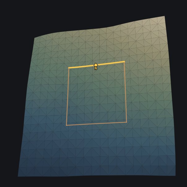
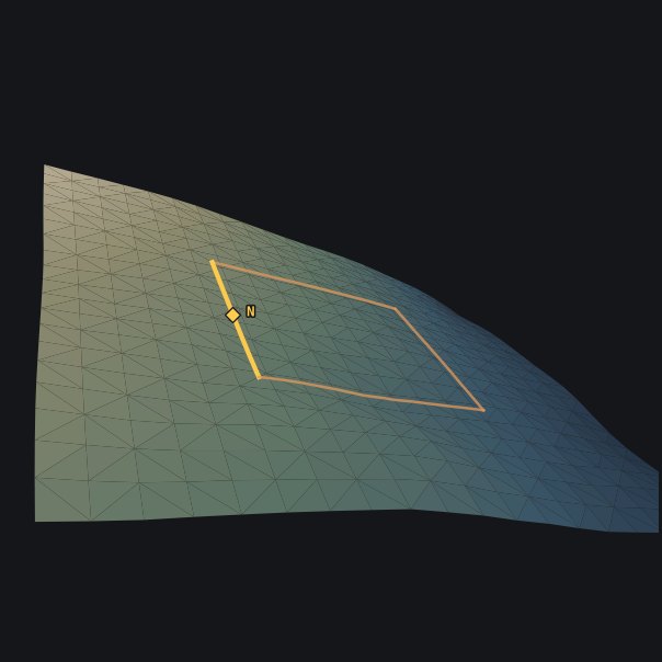
04The computed, rendered surface
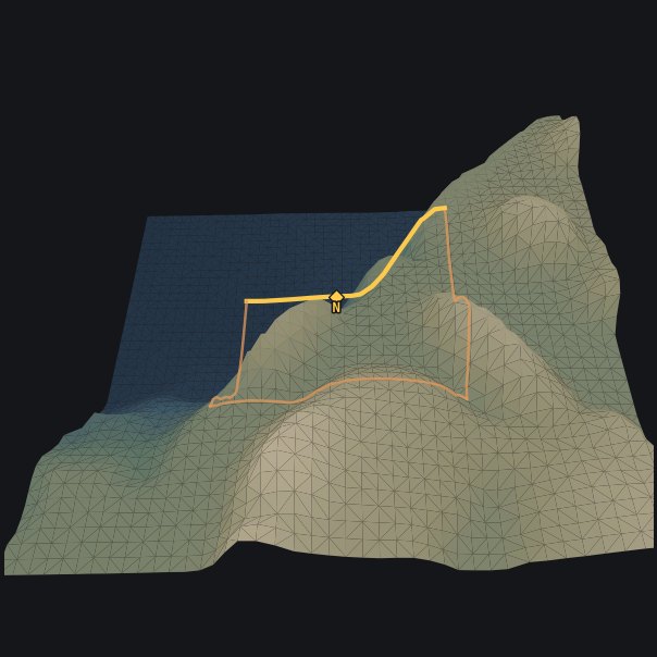
Zoomed far out and map-aligned with plate 01: the site boundary, badge on its marked edge, small within the surrounding terrain.A second, low oblique view of the site in its surroundings, boundary badged.
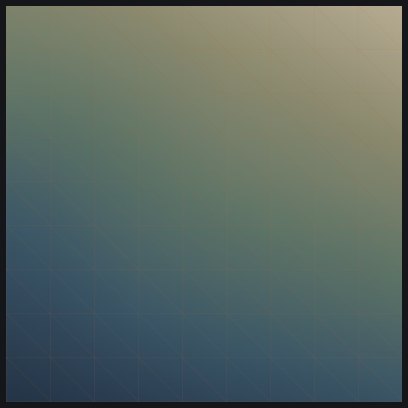
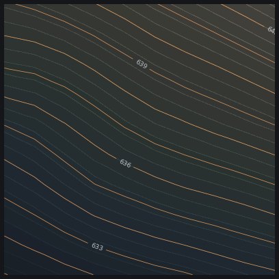
Plate 0 · from ground to model · seven viewsFirst the engine builds the model, then it reads figures from it. The build: the lot from above (01), the elevation points it samples (02), and the Delaunay mesh it triangulates (03), lifted into the 3D surface (04), a slow aerial pass flanked by stills, the left one map-aligned with 01. The supporting tiles at right read that surface off: colored by height (05), contour lines (06), shaded relief (07). The figures below are computed on this modeled surface. Vertical exaggeration ×3.0.
Supporting reads
05 · ELEVATION · 631–643 m
The surface colored by elevation.
06 · CONTOURS
The surface as contour lines.
07 · SHADED RELIEF
The surface lit as shaded relief.
39 ft
Fall across lot
12.9 %
Steepest grade
2,089 ft
Balanced pad
9,160 yd³
Earth moved
~0 yd³
Hauled off-site
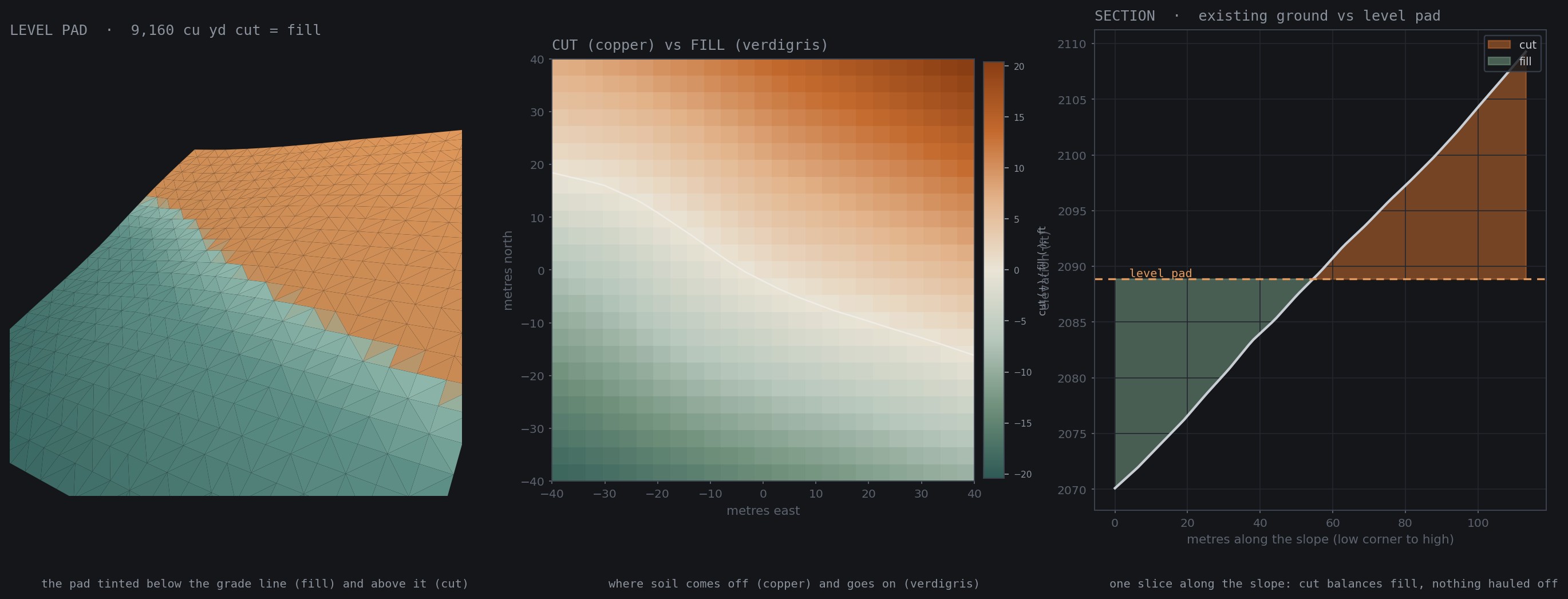
Grading the lot to a level pad: the 3D pad tinted for cut and fill, a cut and fill map, and a cross-section from the low corner to the high.
Plate 1 · grading · 80 × 80 m padGrading the lot to one level building pad. The engine finds the height where the soil cut off the high side exactly fills the low side: 9,160 cubic yards each way, nothing trucked in or hauled out. Copper is cut, verdigris is fill; the section at right runs from the low corner up to the high one.
How to read it: copper is soil cut off the high ground, verdigris is soil filled into the low ground, and the two balance, so no dirt has to leave the site.

The pad

You cut the high side down and fill the low side up until it's level. Put the pad at the balanced grade (2,089 ft) and the dirt you remove matches the dirt you need, so almost nothing leaves the site. On a slope, the trucking is where the money goes.

The dirt

Making the pad moves about 9,160 cubic yards (cut from the high side, placed on the low side), so modeled cut and fill approximately balance. Each figure comes from samples in the public elevation model.

The water

In the modeled surface, runoff moves southwest and concentrates at the low corner. Any drainage intervention would require field verification and site-specific engineering.

02Study 2 · RainwaterWest bluff · San Joaquin River rim · north Fresno

Say your house sits near the rim of this bluff, or you're planning to build one here. Bluffs erode, and 95 feet below runs the San Joaquin. You don't want the foundations creeping toward that edge over the years, so you need to know what every storm does to this ground: which way the rain sheds, where it gathers and cuts, and where it leaves the property. So: where does the rain run?
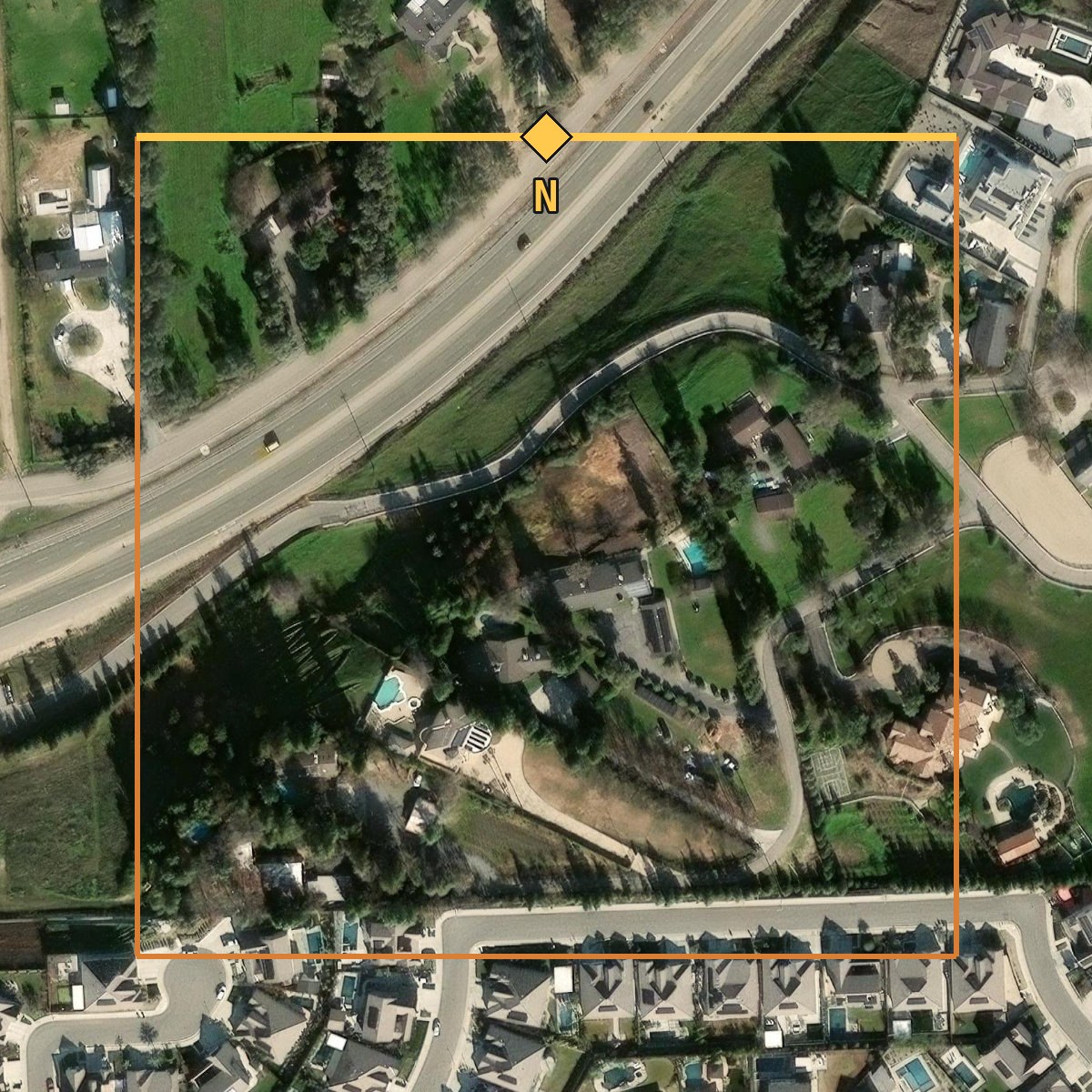
Plain satellite view of the bluff above the San Joaquin, the kind of map view you would pull up before siting houses.
the bluff, from the map
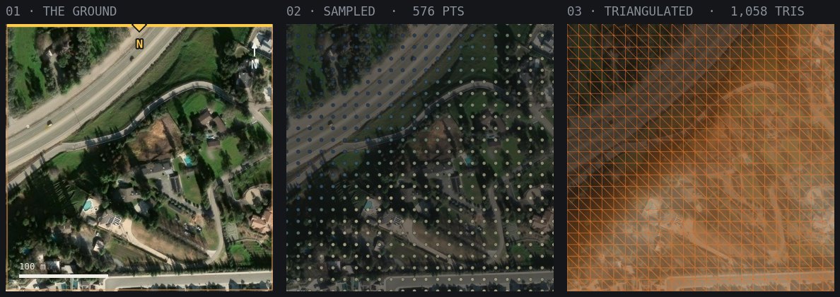
Build maps of the site: the satellite with the study boundary, its marked edge badged with its cardinal letter, the sampled points, and the mesh.
04The computed, rendered surface
Zoomed far out and map-aligned with plate 01: the site boundary, badge on its marked edge, small within the surrounding terrain.A second, low oblique view of the site in its surroundings, boundary badged.
Plate 0 · from ground to model · seven viewsThe same build on the river bluff: satellite (01), the sampled points (02), and the Delaunay mesh (03), lifted into the 3D surface (04), a slow aerial pass flanked by stills, the left one map-aligned with 01, the site outlined in orange inside the surrounding ground. The supporting tiles at right read it off: elevation (05), contour lines (06), shaded relief (07). Vertical exaggeration ×2.9.
Supporting reads
05 · ELEVATION · 92–121 m
The surface colored by elevation.
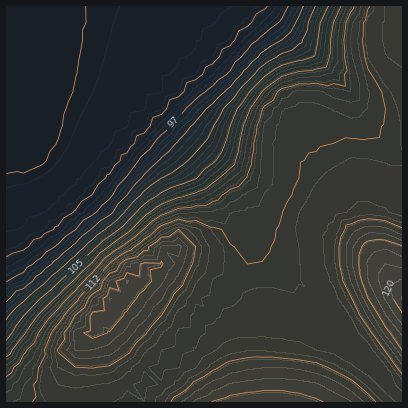
06 · CONTOURS
The surface as contour lines.
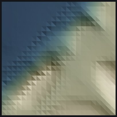
07 · SHADED RELIEF
The surface lit as shaded relief.
95 ft
Fall down bluff
39 %
Steepest grade
NW
Bluff faces
604k gal
Runoff · 1-in storm · 22.2 ac
WNW
Drains to river
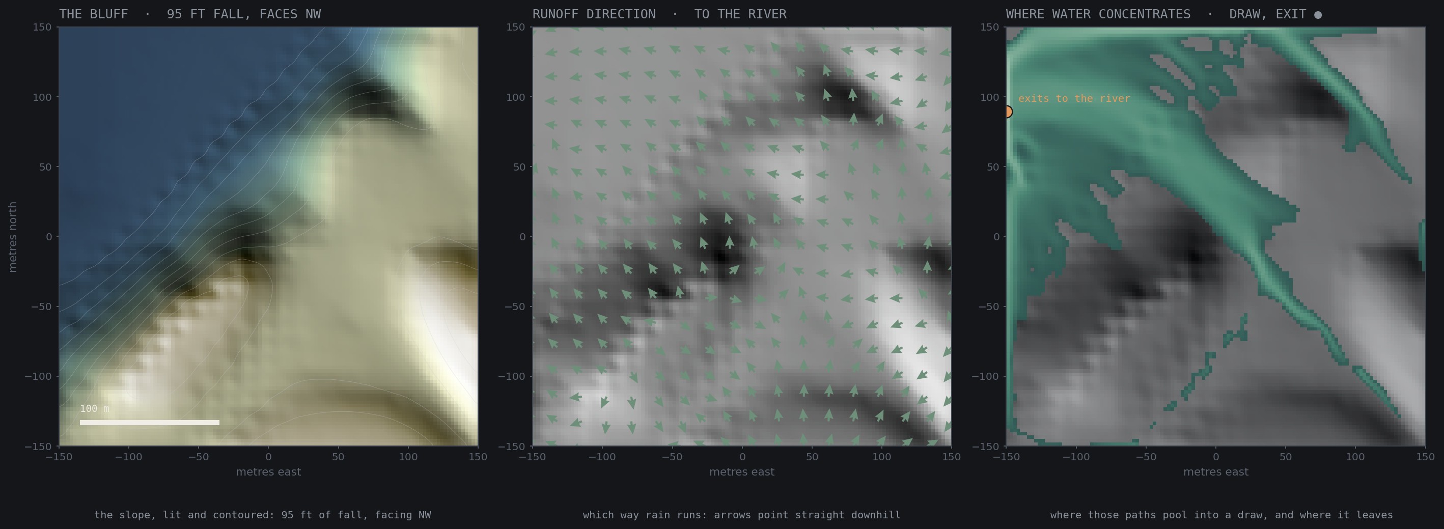
The bluff drainage: shaded relief with contours, downhill runoff arrows, and where flow concentrates into a draw and exits to the river.
Plate 2 · drainage · 300 × 300 mWhere a one-inch storm goes. The bluff lit and contoured (left), the downhill direction at every point (middle), and where those paths pool into a draw and leave toward the river (right, exit marked). About 604,000 gallons run off the modeled slope per inch of rain, assuming zero infiltration — the worst case.
How to read it: the green arrows point downhill the way rain runs, the bright green is where those paths gather into a draw, and the dot marks where the water leaves toward the river.
Plate 2 · animated · a storm over the bluffA storm crossing the modeled bluff: rain lands, gathers into the draws, pools where the ground allows, and drains off toward the river. The study boundary is painted on the ground, its north edge marked in gold with a badge diamond and an N. Illustrative routing on the modeled surface, not calibrated hydrology. Vertical exaggeration ×6.5.

The slope

A steep northwest-facing bluff dropping 95 feet toward the San Joaquin, 39% at the steepest.

The runoff

This water can't be held in place on a 39% face. A 1-inch storm sheds roughly 604,000 gallons off the modeled slope, all of it running downhill.

Where it goes

The runoff gathers into a draw that cuts west-northwest down the bluff and exits toward the river. Anything built near the rim has to respect that draw: it's where the water and the erosion go.

03Study 3 · ReservoirSan Joaquin River gorge · Sierra Nevada · 37.03°N 119.57°W

A regional screening exercise may begin with many possible reservoir sites and incomplete information. This study asks a narrower question of one dry gorge with a single southern outlet: using public 10-meter elevation, what preliminary capacity and dam-height curve does the modeled surface produce? Dam the outlet, and how much would it hold?
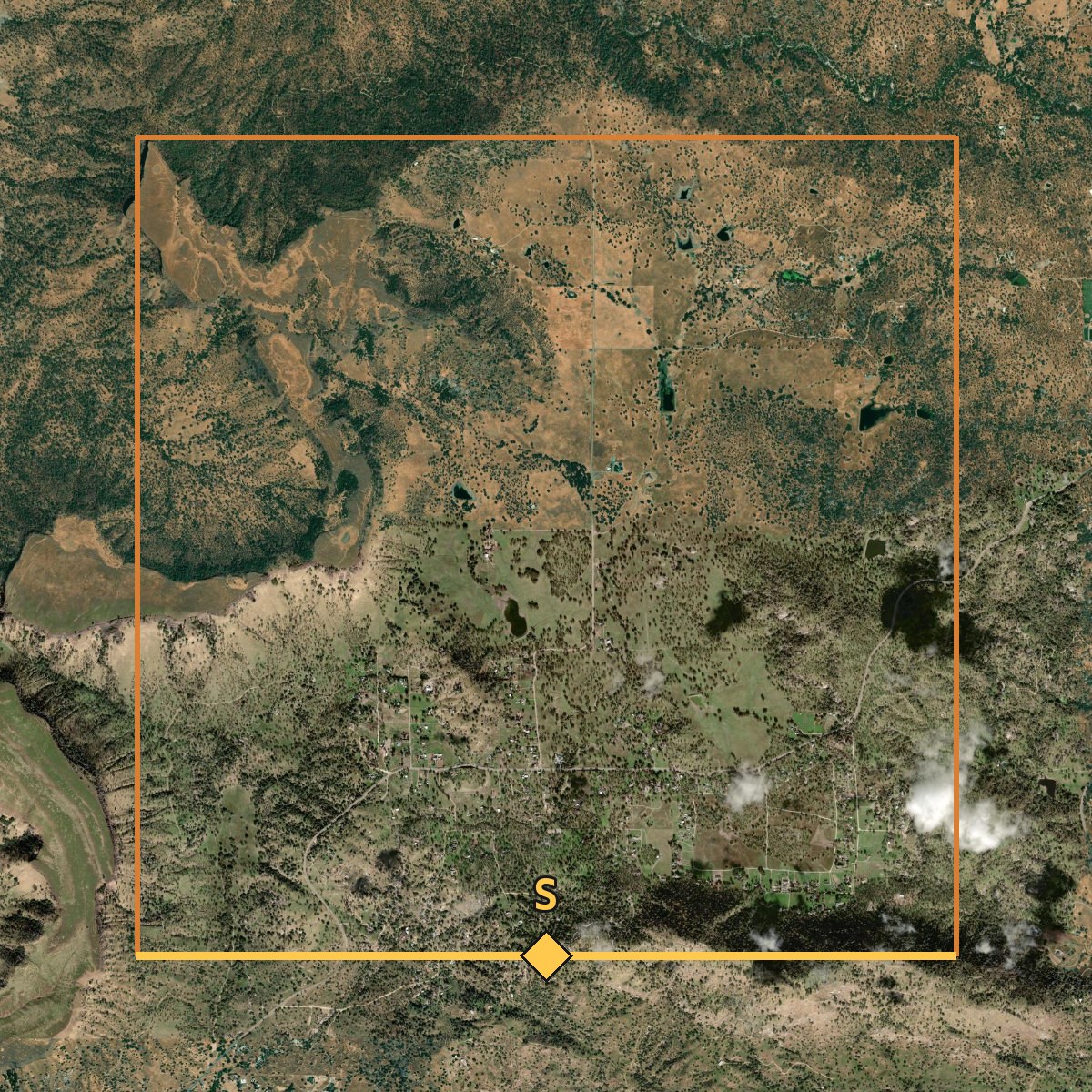
Plain satellite view of the dry gorge and its narrow south outlet, the kind of map view you would pull up before surveying a dam.
the gorge, from the map
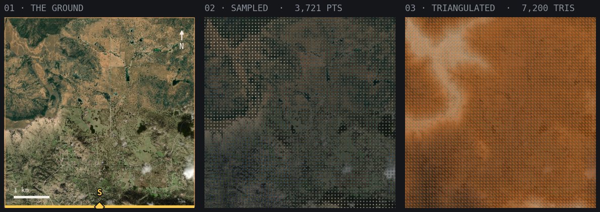
Build maps of the site: the satellite with the study boundary, its marked edge badged with its cardinal letter, the sampled points, and the mesh.
04The computed, rendered surface
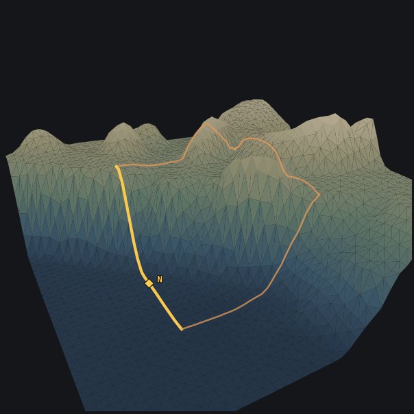
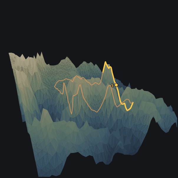
Zoomed far out and map-aligned with plate 01: the site boundary, badge on its marked edge, small within the surrounding terrain.A second, low oblique view of the site in its surroundings, boundary badged.
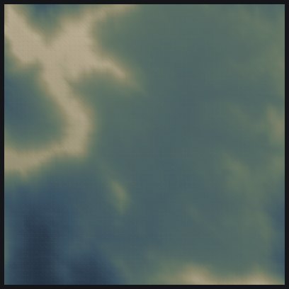
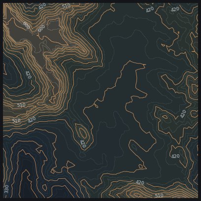
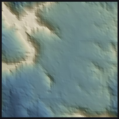
Plate 0 · from ground to model · the canyonThis canyon, built the same way: the Sierra gorge from above (01), 3,721 sampled points (02), and the 7,200-triangle Delaunay mesh (03), lifted into the 3D surface (04), a slow aerial pass flanked by stills, the left one map-aligned with 01, the site outlined in orange inside the surrounding ground. The supporting tiles at right read it off: elevation (05), contours (06), shaded relief (07). The dam and the water it holds come next. Vertical exaggeration ×3.2.
Supporting reads
05 · ELEVATION · 251–617 m
The surface colored by elevation.
06 · CONTOURS
The surface as contour lines.
07 · SHADED RELIEF
The surface lit as shaded relief.
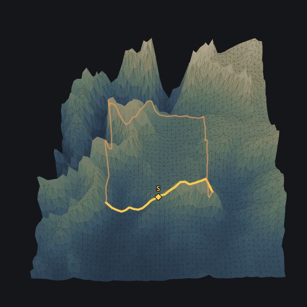
Plate 0 · animated · a storm over the gorgeThe same storm physics over the whole catchment: the drainage network lights up, runoff concentrates, and water collects in the very basin the dam would use. The study boundary is painted on the ground, its south edge marked in gold with a badge diamond and an S. Illustrative routing, not calibrated hydrology. ×3.4 vertical.
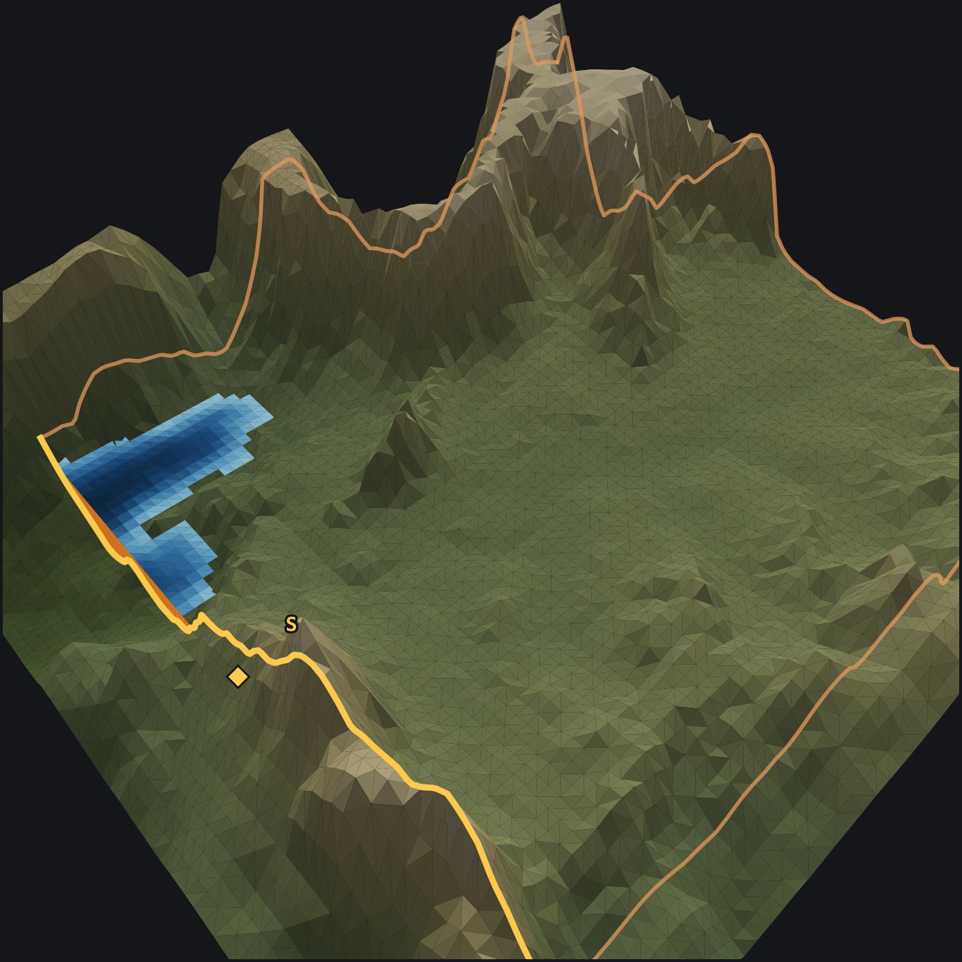
Plate 3 · animated · without the dam, with the damThe case for the site, shown side by side. Without the dam, the drainage runs out the gorge’s one outlet. With it: the dam’s footprint appears first as a phantom, drops into place, and the reservoir fills behind it while the stream below runs dry. The reservoir is the flooded basin the engine computes, not a drawn shape. ×3.4 vertical.
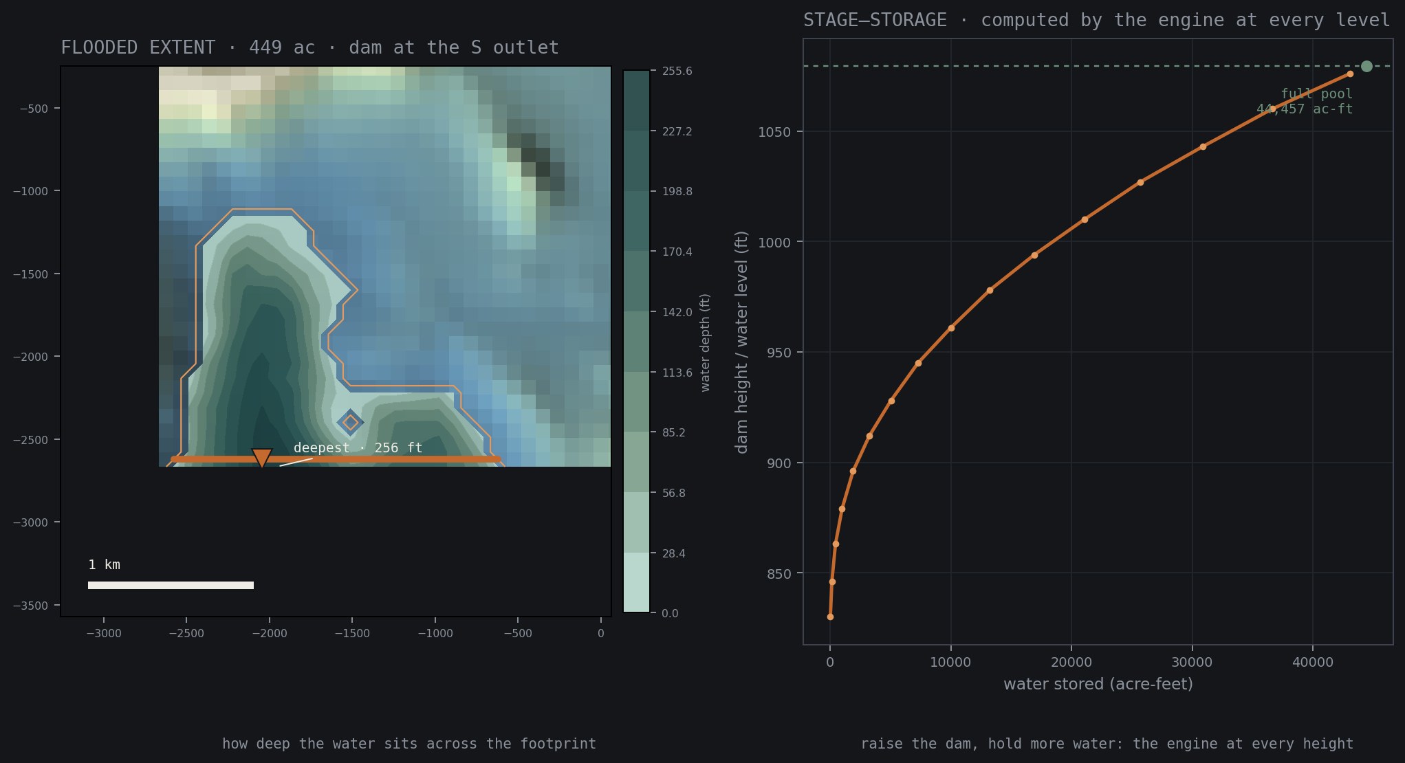
The canyon at full pool from the air: the impounded reservoir shaded by depth (dark where deepest) behind the orange dam wall at the south outlet, the study boundary marked in copper with its south edge in gold.The flooded extent shaded by water depth with the dam and deepest point marked, and the engine's stage-storage curve, capacity at every waterline.
Plate 4 · reservoir · full poolIn the model, a dam across the south outlet fills the gorge to 44,457 acre-feet. The canyon at full pool from the air (left), the flooded footprint shaded by depth with the dam and deepest point marked (middle), and the stage-storage curve at each modeled waterline (right). Capacity is integrated below the waterline from public 10-meter elevation: a preliminary estimate, not a design survey.
How to read it: the orange wall is the dam, darker blue is deeper water, and the curve on the right shows how much the reservoir holds as the dam is built taller.
44,457 ac-ft
Full-pool capacity
256 ft
Dam height
449 ac
Surface at full pool
14.5 B gal
Water impounded
0.9 mi
Reservoir reach

The basin

A dry Sierra gorge that falls to a single narrow outlet on the south. Close that notch with a 256-foot dam and the canyon behind it becomes a reservoir, held on the other three sides by its own rim.

The modeled capacity

At the selected full-pool elevation, the model yields 44,457 acre-feet, about 14.5 billion gallons. The stage–storage curve reports the estimated capacity at successive waterlines.

What the estimate supports

At this resolution, the result is a preliminary capacity and dam-height estimate for comparing sites. It is not a design value and still requires surveyed elevation, calibrated hydrology, and engineering review.

Why this exists

This is a portfolio demonstration rather than a product. It combines Planar—a standard-library C++ geometry workbench built on a hand-written foundation and later expanded with coding agents—with a geospatial platform I architected, applied to three Sierra and foothill sites.

Neither system was built for terrain. The geospatial platform originated as a county data pipeline; Planar began with geometric primitives, polygon operations, and ear-clipping triangulation. Delaunay, Voronoi, and terrain came later.

Public USGS elevation goes in; the geometry engine turns it into a triangulated surface; earthwork, drainage, and reservoir calculations run on that surface; a real lot boundary can come from the platform. The foundational geometry primitives, polygon operations, and original ear-clipping implementation are hand-written. Coding agents later substantially revised the ear clipper and implemented the current Delaunay/Voronoi and terrain layers under my direction and review. I designed the platform architecture, schema, scoring, and test gates; coding agents produced most of its Python implementation.
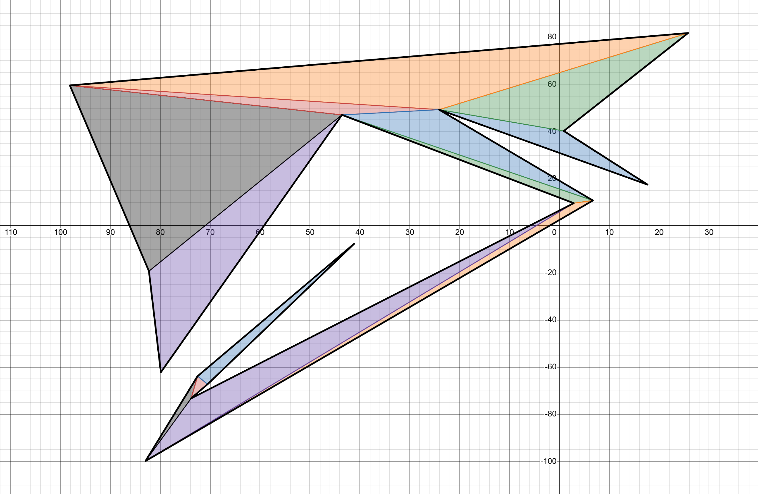
The geometry engine's triangulation export rendered in its Desmos viewer: a spiky 15-vertex polygon ear-clipped into 13 colored triangles on graph paper.
the geometry engine's desmos viewer · a 15-vertex polygon in → 13 triangles out
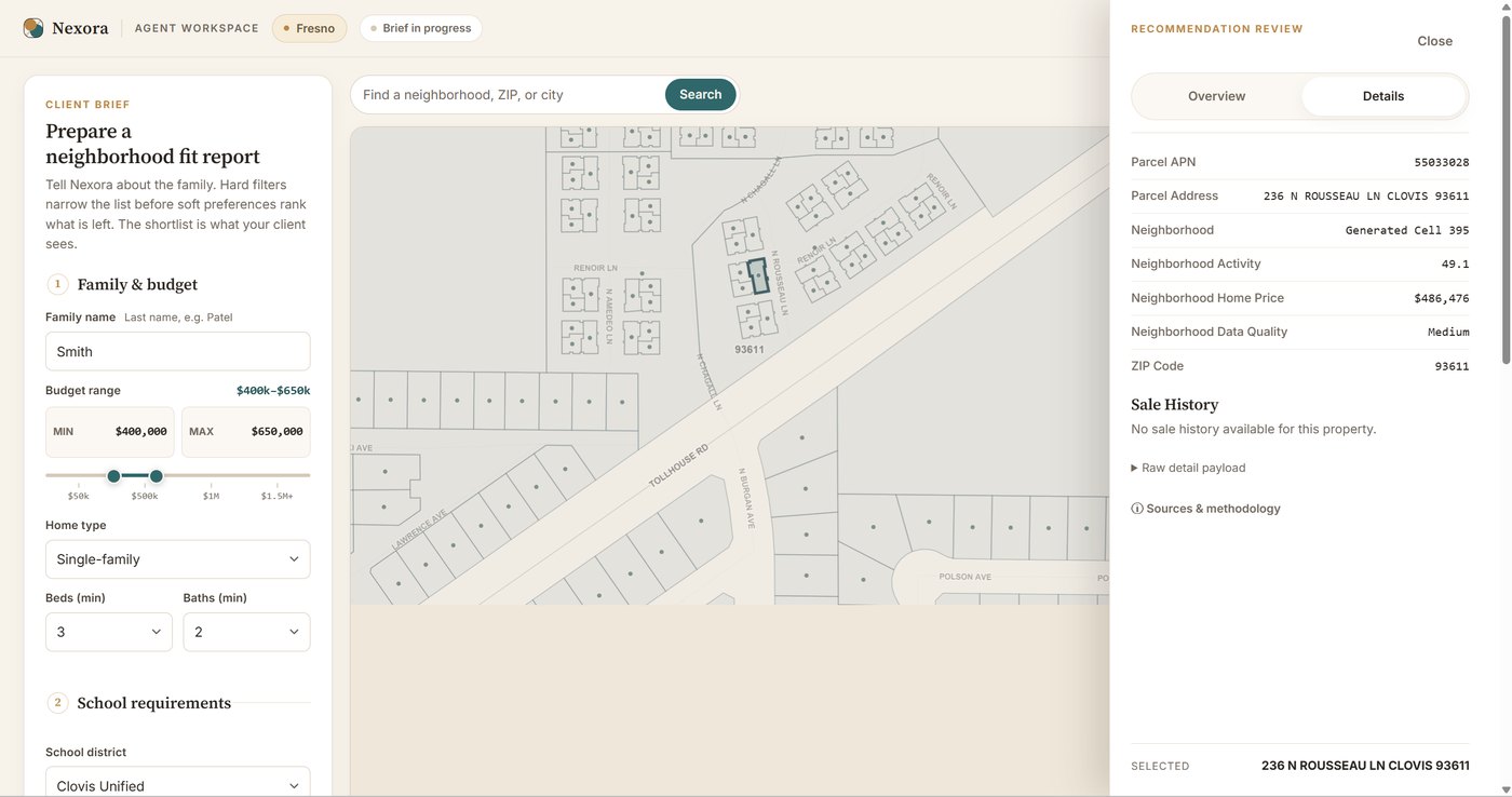
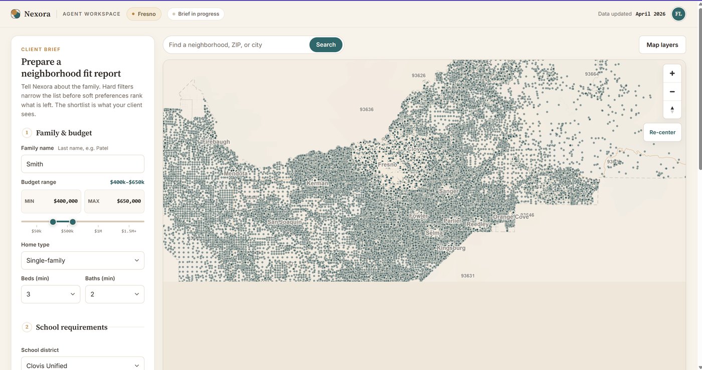
The geospatial platform's map of Fresno County rendered as one dot per parcel.
the platform's map of fresno county, parcel by parcel · the front end to precomputed scores
Engine 01planar-geometry · C++ · hand-written foundation + later agent assistance

A bare terminal: numbers in, numbers out. Every surface below is built from what it computes.

$ delaunay_driver --random --random-count=1500 --coord-max=1000

Generated 1500 random points within [-1000, 1000].
Input sites:            1500
Delaunay triangles:     2976
Voronoi vertices:       2976
Voronoi finite edges:   4453
Delaunay validation:    passed
1,500 random points → 2,976 Delaunay triangles and the full Voronoi dual, validated, in 0.09 s

Those counts are the summary line, not the computation. In that 0.09 s the engine constructs every one of those objects — each triangle, each Voronoi vertex and edge, coordinates and adjacency — and then verifies the whole structure against the Delaunay condition before printing passed. The terrain surfaces above are these same structures, built from elevation samples instead of random points.
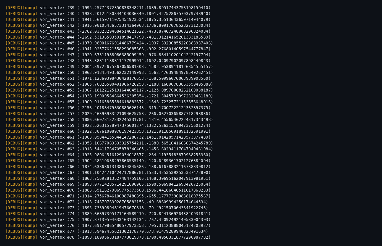
Debug dump mid-scroll: dozens of Voronoi vertices, each printed as a 20-digit coordinate pair, scrolling past.
the dump behind the summary line · every voronoi vertex, coordinates and all · a separate debug run
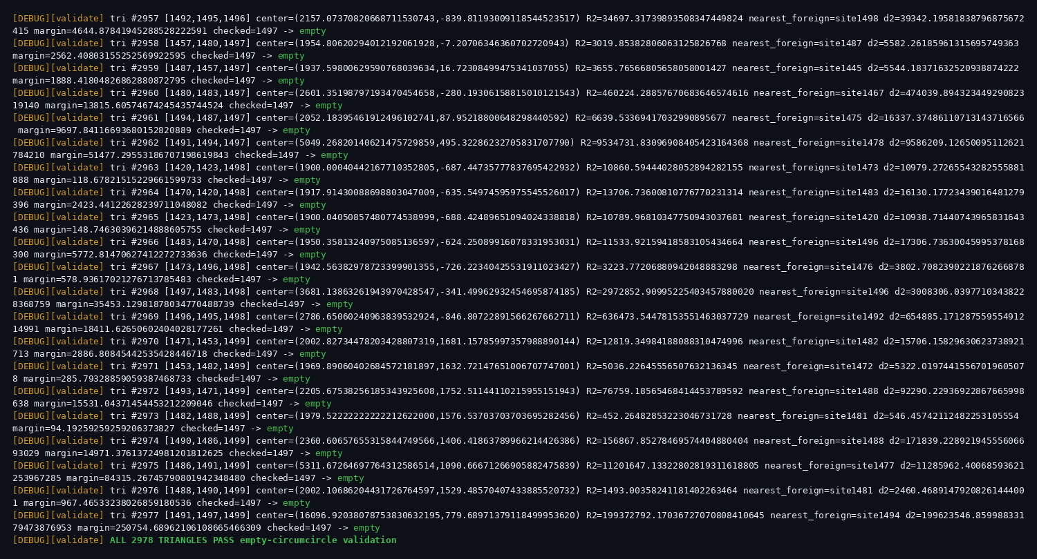
Empty-circumcircle validation trace: per-triangle circumcenter, radius, nearest foreign site, and margin, ending in ALL TRIANGLES PASS.
the validation validating · one empty-circumcircle check per triangle, margins printed → all pass · another debug run
Point twoMinus1  = p2 - p1;
Point thisMinus1 = *this - p1;

// scale epsilon to the problem size
double scale = max({1.0,
    fabs(twoMinus1.get_x()), fabs(twoMinus1.get_y()),
    fabs(thisMinus1.get_x()), fabs(thisMinus1.get_y())});
double eps = 1e-12 * scale;

// 1) collinear?
if (fabs(cross(twoMinus1, thisMinus1)) > eps) return false;
// 2) between-ness via projection
double proj = dot(thisMinus1, twoMinus1);
if (proj < -eps) return false;
one predicate, hand-written · is a point on this segment, within a scaled tolerance
$ ./interview_demo --run-sample-demo

Sample polygon
Vertices:
(-4,0)
(-1,3)
(3,4)
(5,1)
(2,-3)
(-3,-4)
Area: 46
Concave/Convex? Convex

Triangulation:
{(-3,-4), (-4,0), (-1,3)}
Center: (-2.66667,-0.333333)
Area: 7.5
{(-3,-4), (-1,3), (3,4)}
Center: (-0.333333,1)
Area: 13
...
one polygon, under the hood · vertices in → area, convexity, and an ear-clipping triangulation out
Engine 02geospatial platform · Python

The same approach on different material: county records go in, versioned scores come out, and the map is just the interface.
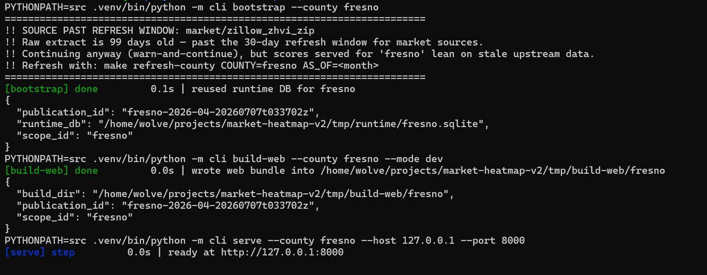
Terminal run of the real pipeline: bootstrap, build-web, and serve steps with timings, plus a stale-data warning banner.
the real pipeline · bootstrap → build → serve — and it flags stale upstream data instead of hiding it
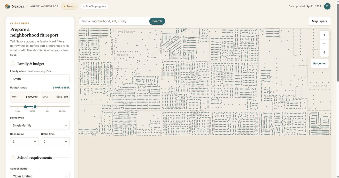
The same map zoomed to Clovis street level, each dot a parcel on a named street.
the same data, three zooms down · every dot a parcel on a named street
A single-parcel detail panel: APN, address, neighborhood cell, modeled price, and a data-quality label.
one parcel · APN, neighborhood cell, modeled price — with the data-quality label right beside it
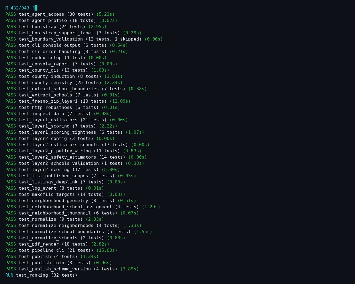
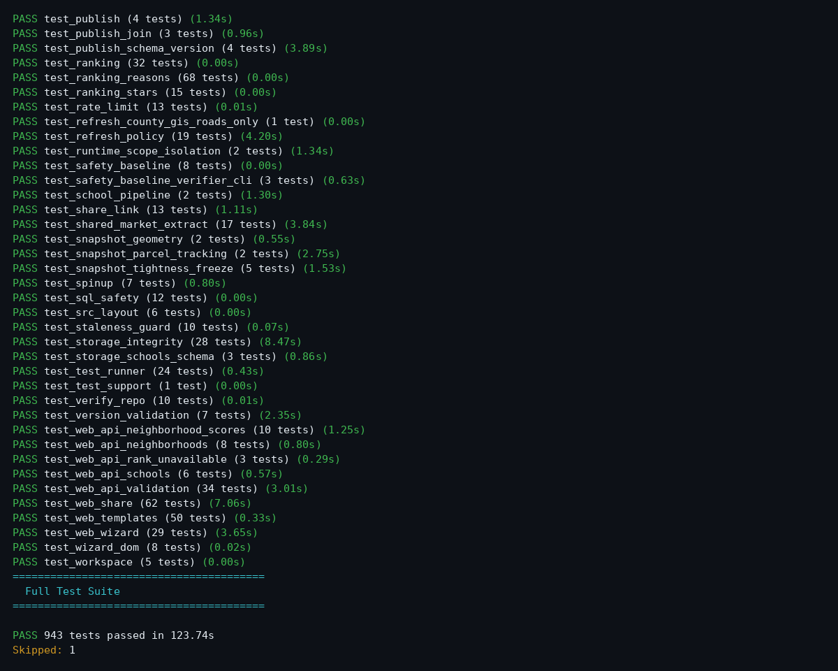
The platform's Python test suite mid-flight at the pictured commit: 432 of 943 tests complete, dozens of PASS lines with per-suite timings, test_ranking currently running.
the suite at the pictured commit · 432/943, per-suite timings, test_ranking in the chamber
The end of the pictured run: the web, storage, and safety suites passing, then the tally — 943 tests passed in 123.74 seconds, 1 skipped.
the pictured run · 943 tests passed in 123.74 s · 56 modules at that commit

How this was made

01 · elevation

Real USGS 10-meter elevation, sampled across each site: 100 points on the pad, 576 on the bluff, and 3,721 across the reservoir basin.

02 · surface

The points are triangulated into a continuous surface (a TIN) by a standard-library C++ geometry workbench built on a hand-written foundation and later expanded with coding agents. 162, 1,058, and 7,200 triangles, exact to Euler's formula.

03 · analysis

From that surface: cut and fill balanced to a pad, and rainfall routed downhill neighbor-to-neighbor to find where water concentrates.

The 3D views are plots of the mesh underneath. Triangulation, balanced cut and fill, reservoir capacity, and drainage analysis ran locally through the Planar/terrain toolchain; I directed and reviewed the agent-assisted terrain extension. Elevation comes from public USGS data, and the visualizations use external plotting libraries.
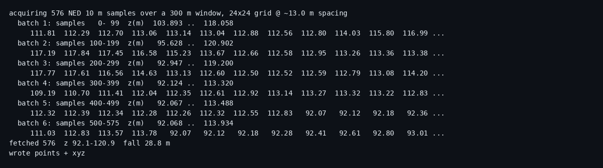
Terminal log of 576 USGS NED 10-meter elevation samples arriving in six batches over a 300-meter window, with per-batch elevation ranges.
step 01, live · 576 elevation samples arriving batch by batch · the bluff
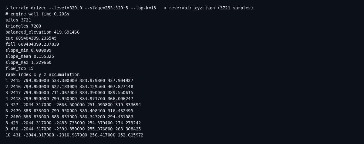
Terminal run over the reservoir basin: 3,721 sites triangulated into 7,200 triangles in 0.206 seconds, with slope statistics and the top flow-accumulation points.
step 02 · 3,721 samples → 7,200 triangles in 0.206 s, slope and flow read off the mesh · the canyon
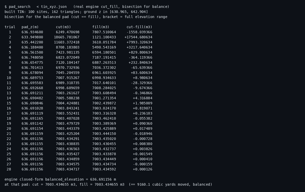
Bisection table converging on the balanced pad: 28 trials narrowing cut-minus-fill from thousands of cubic meters to a fraction, ending at 9,160.1 cubic yards, matching the engine's closed-form answer.
step 03 · 28 bisection trials to a 0.0001 m³ residual, and the engine’s closed-form answer agrees: 9,160.1 yd³ · the pad
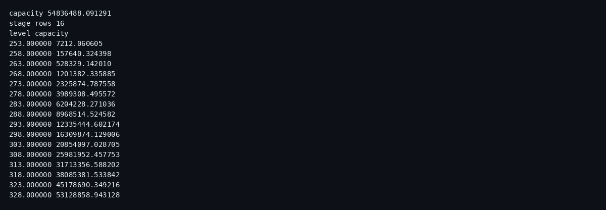
Stage-storage sweep: capacity computed at 16 waterlines from 253 to 328 meters, totaling 54,836,488 cubic meters at full pool.
step 03 · the stage–storage sweep, 16 waterlines → 54,836,488 m³ (44,457 acre-ft) · the reservoir
County GIS · layer ready

It runs on the same engine as my county GIS platform, so a lot boundary can come from official parcel data, and either study runs on any parcel in the county from its address alone, or any given coordinate boundary, provided elevation data exists.

A demonstration of the method on real public data, not a licensed survey or construction document. Locations are approximate; satellite imagery courtesy Esri World Imagery. Ten-meter elevation supports preliminary comparison only. The pipeline can also accept a surveyed point cloud, but that path is not demonstrated here.